Contents

close all;
clear all;
CSVM_pattern
warning off;

Formulate DC State-Space model_dc

A_dc = [[0       -1/L_dc];
        [1/C_dc  -1/(C_dc*R_dc)]];

B_dc = [1.5/L_dc; 0];

C_dc_ = [0 1];

D_dc = 0;


% %% dimension declaration
% [m1, n1] = size(C_dc_);
% [n1, n_in] = size(B_dc);
%
% %% augmented model creation
% A_e = eye(n1+m1, n1+m1);
% A_e(1:n1, 1:n1) = A_dc;
% A_e(n1+1:n1+m1, 1:n1) = C_dc_ * A_dc;
%
% B_e = zeros(n1+m1, n_in);
% B_e(1:n1, :) = B_dc;
% B_e(n1+1:n1+m1, :) = C_dc_ * B_dc;
%
% C_e = zeros(m1,n1+m1);
% C_e(:, n1+1:n1+m1) = eye(m1,m1);
%
%
% Buck_C = ss(A_e,B_e,C_e,D_dc);
Buck_C = ss(A_dc,B_dc,C_dc_,D_dc);
Buck_D = c2d(Buck_C, t_sample,'zoh');
model_dc = LTISystem(Buck_D);

U_dc_ref = 400;
xref = [U_dc_ref/R_dc U_dc_ref]';

model_dc.x.with('reference');
model_dc.x.reference = xref;
% yref = 400;
% model_dc.y.with('reference');
% model_dc.y.reference = yref;
%model_dc.with('integrator');

Give DC constraints

% hard constraints
% set constraint
% xconst = 500;
% P = Polyhedron('lb', [-0; -0], 'ub', [500; 500]);
% model_dc.x.with('initialSet');
% model_dc.x.initialSet = P;

 model_dc.x.max = [50; 500];  % constraint formulation
 model_dc.x.min = [0; 0];
%  model_dc_ac.y.max = [500];
%  model_dc_ac.y.min = [0];

  model_dc.u.max = [600];
  model_dc.u.min = [0];
%   model_dc.u.with('deltaMin');
%   model_dc.u.with('deltaMax');
%   model_dc.u.deltaMax = 750;
%   model_dc.u.deltaMin = -750;

% model_dc.y.with('softMax');
% model_dc.y.with('softMin');
% model_dc.x.with('softMax');
% model_dc.x.with('softMin');
% model_dc.u.with('softMax');
% model_dc.u.with('softMin');


% soft constraints
model_dc.u.penalty = OneNormFunction( 1e-6 );
model_dc.x.penalty = OneNormFunction( diag([1, 1]));
% model_dc.u.with('deltaPenalty');
% model_dc.u.deltaPenalty = QuadFunction( 1e-8 );
%model_dc.x.penalty = QuadFunction(diag([1000, 1000]));
% model_dc.y.penalty = OneNormFunction( 1 );

U0_result_matrix = [];
Trees = [];
maxiter = 2;
for i=1:maxiter

Set DC horison and formulate contrl rules

    N_dc = i;
    mpc = MPCController(model_dc, N_dc);
    expmpc_dc = mpc.toExplicit();

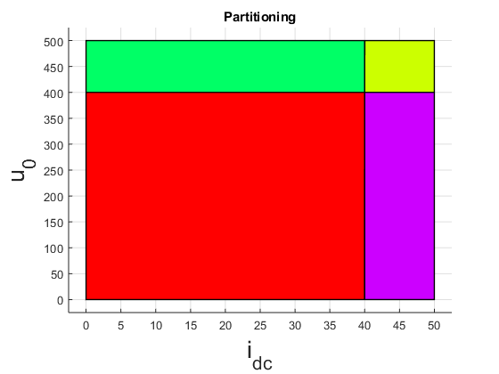
    if (i == maxiter)
        figure
        expmpc_dc.partition.plot();
        title('Partitioning')
        xlabel('i_{dc}','FontSize',20)
        ylabel('u_{0}','FontSize',20)
    end

mpt_plcp: 6 regions

mpt_plcp: 13 regions

Constructing binary tree

    Tree = BinTreePolyUnion(expmpc_dc.optimizer);
    %genvarname('tree', num2str(i)) =  tree;

    save(genvarname(['Tree',  num2str(i)],'Tree'));

%     %% Create fancy plots
%
%     title(Partitioning)
%     xlabel('x_1')
%     ylabel('x_2')
%     print -deps SimpleExplicit_Buck_Partition
%
%     %% Simulate
%
%     loop = ClosedLoop(expmpc_dc, model_dc);
%
%     x0 = [0 0 ]';
%     u0 = 400;
%     Nsim = 40e3;
%     %data = loop.simulate(x0, Nsim, 'x.reference', repmat(xref, 1, Nsim));
%     %data = loop.simulate(x0, Nsim, 'u.previous', u0);
%     data = loop.simulate(x0, Nsim);
%     figure
%     subplot(2, 1, 1);hold on
%     plot(1:Nsim, data.X(1,1:Nsim),'g', 'linewidth', 2);
%     plot(1:Nsim, data.X(2,1:Nsim),'k', 'linewidth', 2);
%     %plot(1:Nsim, data.X(3,1:Nsim),'r', 'linewidth', 2);
%     plot( 1:Nsim, xref(1)*ones(1,Nsim), 'k--', 1:Nsim, xref(2)*ones(1,Nsim), 'k--');
%     plot( 1:Nsim, model_dc.x.max(1)*ones(1,Nsim), 'r--', 1:Nsim, model_dc.x.max(2)*ones(1,Nsim), 'r--');
%     legend('X1','X2','X3');
%
%     subplot(2, 1, 2);
%     plot(1:Nsim, data.U(:,1:Nsim),'b', 'linewidth', 2);hold off
%     legend('U');
%
%     figure
%     plot(1:Nsim, data.Y(:,1:Nsim),'b', 'linewidth', 2);
%     legend('Y');

Found 7 unique hyperplanes (out of 23)
Determining position of 6 regions w.r.t. unique hyperplanes...
...done in 0.1 seconds.
Discarding 4 outer boundaries.
Considering 3 candidates for separating hyperplanes.
Constructing the tree...
...done in 0.0 seconds.
Depth: 3, no. of nodes: 4

Found 12 unique hyperplanes (out of 50)
Determining position of 13 regions w.r.t. unique hyperplanes...
...done in 0.2 seconds.
Discarding 4 outer boundaries.
Considering 8 candidates for separating hyperplanes.
Constructing the tree...
...done in 0.1 seconds.
Depth: 4, no. of nodes: 9

Export DC explicit controller to C

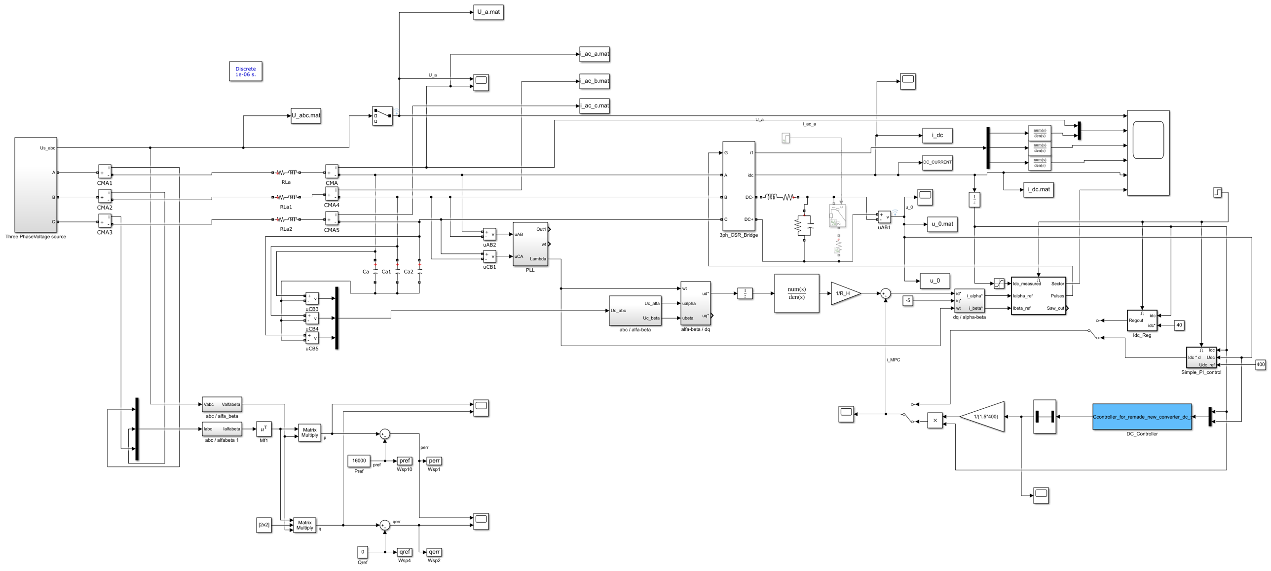
    clear dir_name;
    clear file_name;
    dir_name = 'remade_new_converter_dc/new_converter_explicitMPC_dc';
    file_name = 'EMPCcontroller_for_remade_new_converter_dc';
    expmpc_dc.exportToC(file_name,dir_name);


    % Compile S-Function
    p = [pwd,filesep,dir_name,filesep];
    mex(['-LargeArrayDims -I',dir_name],[p,file_name,'_sfunc.c'],[p,file_name,'.c']);

    % Set the source files in the Simulink scheme
    simple_explicit_buck;
    str = sprintf('"%s%s_sfunc.c" "%s%s.c"',p,file_name,p,file_name);
    set_param('simple_explicit_buck','CustomSource',str);
    set_param('simple_explicit_buck/DC_Controller','FunctionName',[file_name,'_sfunc']);

Output written to "D:\CloudVIRT\2018_ActaHung_EMPC_for_CSI\Matlab\EMPC_Implementation_no_figures\remade_new_converter_dc/new_converter_explicitMPC_dc\EMPCcontroller_for_remade_new_converter_dc.c".
C-mex function written to "D:\CloudVIRT\2018_ActaHung_EMPC_for_CSI\Matlab\EMPC_Implementation_no_figures\remade_new_converter_dc/new_converter_explicitMPC_dc\EMPCcontroller_for_remade_new_converter_dc_mex.c".
Building with 'MinGW64 Compiler (C)'.
MEX completed successfully.

Output written to "D:\CloudVIRT\2018_ActaHung_EMPC_for_CSI\Matlab\EMPC_Implementation_no_figures\remade_new_converter_dc/new_converter_explicitMPC_dc\EMPCcontroller_for_remade_new_converter_dc.c".
C-mex function written to "D:\CloudVIRT\2018_ActaHung_EMPC_for_CSI\Matlab\EMPC_Implementation_no_figures\remade_new_converter_dc/new_converter_explicitMPC_dc\EMPCcontroller_for_remade_new_converter_dc_mex.c".
Building with 'MinGW64 Compiler (C)'.
MEX completed successfully.

Simulate model

    open_system('simple_explicit_buck');
    sim('simple_explicit_buck');

Found algebraic loop containing: 
<a href="matlab:open_and_hilite_hyperlink ('simple_explicit_buck/Subsystem/ModI_Lim','error')">simple_explicit_buck/Subsystem/ModI_Lim</a>
<a href="matlab:open_and_hilite_hyperlink ('simple_explicit_buck/Subsystem/SatDyn/LowerRelop1','error')">simple_explicit_buck/Subsystem/SatDyn/LowerRelop1</a> (discontinuity)
<a href="matlab:open_and_hilite_hyperlink ('simple_explicit_buck/Subsystem/SatDyn/Switch2','error')">simple_explicit_buck/Subsystem/SatDyn/Switch2</a> (algebraic variable) (discontinuity)

Found algebraic loop containing: 
<a href="matlab:open_and_hilite_hyperlink ('simple_explicit_buck/Subsystem/ModI_Lim','error')">simple_explicit_buck/Subsystem/ModI_Lim</a>
<a href="matlab:open_and_hilite_hyperlink ('simple_explicit_buck/Subsystem/SatDyn/LowerRelop1','error')">simple_explicit_buck/Subsystem/SatDyn/LowerRelop1</a> (discontinuity)
<a href="matlab:open_and_hilite_hyperlink ('simple_explicit_buck/Subsystem/SatDyn/Switch2','error')">simple_explicit_buck/Subsystem/SatDyn/Switch2</a> (algebraic variable) (discontinuity)

Store results

    U0_result_matrix = [u_0.Data U0_result_matrix];

    clear mpc;
    clear expmpc_dc;
    clear Tree;

    disp(i);

     1

     2

end

Save results to file

save('Resultmatrix.mat','U0_result_matrix')
time = u_0.Time; save('Resultmatrix_time.mat','time'); clear time;
save('Treesmatrix','Trees')

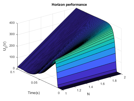
Plot all results

load('Resultmatrix');
D = U0_result_matrix;
load('Resultmatrix_time');
t = time;
res = 1000;
res_U0_result_matrix = [];
j = 1;
i = size(D,2);
res_D = [];
for j=1:i
    res_D = [D(1:res:end,j) res_D];
end

res_t = t(1:res:end);

iteration = 1:1:i;

if (size(iteration,2) > 1)
    figure
    surf(iteration,res_t,res_D)
    title('Horizon performance')
    xlabel('N')
    ylabel('Time(s)')
    zlabel('U_0(V)')
end

Published with MATLAB® R2019a